House Price Analysis and Prediction
Using SAS Enterprise Miner
Table of Contents
2 Exploratory
Data Analysis (EDA)
4 Model
Construction, Optimization and Validation
4.3 Model
Comparison (Regression and GB model)
1
Business Case
A
property developer that specializes in the residential property sector is
planning to embark on its next project in the area. The management of the
company would like to know the type of house, location and price that are
marketable. It is vital for the company to have insights regarding this to
better position itself to meet the market demand and reduce the risk of
property overhang.
In
this case study we will look at house sales data from King Country in the state
of Washington, USA. The relevant transaction data is obtained from Kaggle
website and the details of the dataset is described in
the scope of work section.
1.1
Objectives
A number of objectives
have been identified to achieve the aim of this study. They are described
below:
1. To
visualize the acquired data using Tableau and identify trend or variation in
house price by geographical location and different physical attributes.
2. To
predict house price from its geographic location and physical attributes using
suitable machine learning algorithms via SAS Enterprise Miner.
3. To
provide strategies and recommendation to the business from the insights gained
in the analysis.
1.2
Dataset
A
summary of the different variables that is included in the final dataset is
described in Table 1
below. The dataset is acquired from Kaggle website and can be accessed through:
https://www.kaggle.com/harlfoxem/housesalesprediction
Table 1: Summary of the dataset that will be
used in the study.
|
Variable |
Description |
|
id |
Transaction ID for each house sales |
|
date |
Date of transaction |
|
price |
Price of house sold |
|
bedrooms |
Number of bedrooms |
|
bathrooms |
Number of bathrooms |
|
sqft_living |
Size of living room in square-feet |
|
sqft_lot |
Size of lot (land) in square-feet |
|
floors |
Number of rooms |
|
waterfront |
Waterfront facing house (1 = yes, 0 = no) |
|
view |
Rank of view from the house (0, bad – 4, excellent) |
|
condition |
Condition of the house (1, bad – 5, excellent) |
|
grade |
Level of craftsmanship, material, design, construction (1,
bad – 13, excellent) |
|
sqft_above |
Size of house space above the ground level in square-feet |
|
sqft_basement |
Size of basement in square-feet |
|
yr_built |
The year that the house was built in |
|
yr_renovated |
The year that house was renovated |
|
zipcode |
Zipcode area of the house |
|
lat |
Latitude |
|
long |
Longitude |
The
software used for data mining purposes in this study are Tableau and SAS
Enterprise Miner.
2 Exploratory Data Analysis (EDA)
The dataset for this study contains 19 variables and they have been described in Table 1 under the Error! Reference source not found. and the data type is presented in Figure 2 below. For the modelling study which aims to predict the house price, 15 variables will be utilized namely, price, bedroom, bathrooms, sqft_living, sqft_lot, floors, view, condition, grade, sqft_above, sqft_basement, lat and long. Each variable is explored using descriptive statistics, histograms, and correlation plots to identify any inconsistencies, understand the overall data distribution for each independent variable and their relationship with the target variable – price.
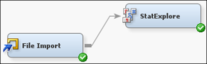
Figure 1: Exploratory data analysis is performed using the StatExplore node.
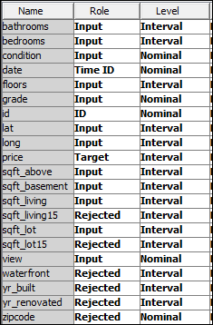
Figure 2: Data types of the variables found in the dataset.
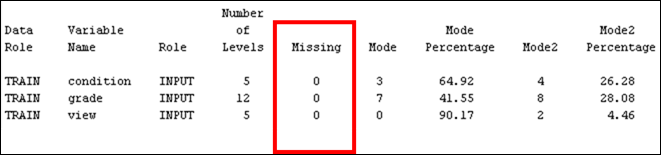
Figure 3: Descriptive statistics for nominal data.
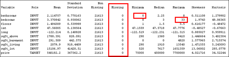
Figure 4: Descriptive statistics for interval data. Red box indicates suspicious minimum number of bathrooms, and maximum number of bedrooms.

Figure 5: Distribution of each variable. Red box indicates the target variable – price that is heavily skewed to the right.
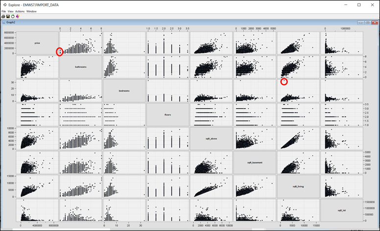
Figure 6: Correlation matrix for price, bedrooms, bathrooms, floors, sqft_above, sqft_basement, sqft_living and sqft_lot. Red box indicates potential outliers.
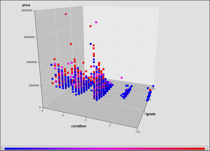
Figure 7: Correlation between price, condition, grade, and view scores.
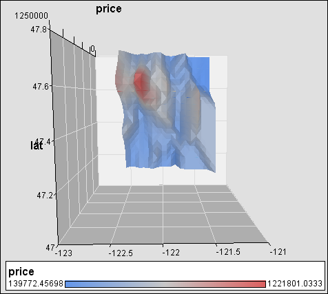
Figure 8: House price variation against latitude and longitude position.
Some observations can be made from the EDA:
· From
the descriptive statistics, it can be observed that there are no missing values
in the dataset. Total number of observations are 21613, which corresponds to
the total number of house sales transaction recorded in the county from May
2014 – May 2015.
· Figure
4 shows that there are observations
with 0 bathrooms and 33 bedrooms. As each residential property
should have at least 1 bathroom to be habitable, records with 0 bathrooms can
be treated as outlier. 0 number of bedrooms can still be acceptable as it may
refer to studio concept units. However, the observation showing 33 number of
bedrooms is suspicious. This observation coincides with a sqft_living of
1620 sqft as highlighted in the red circle from the correlation plot in Figure
6. Since it is not possible to have
such scenario, this observation is also treated as an outlier.
· The
distribution of price is heavily skewed to the right. This needs to be
handled as linear regression will be employed for house price prediction.
Appropriate data transformation technique such as log transformation should be
applied to ensure that assumptions for linear regression (heteroscedasticity and
normality of error terms, linear relationship between dependent and independent
variables) are met.
· From
visual inspection, it can be observed that there is positive correlation
between price and most of the independent variables as shown in Figure
6 and Figure
7. However, the same cannot be interpreted
for the relationship between price and floors and sqft_lot.
· Price
varies
with location. Figure
8 shows that price generally
increases towards the North West with a clear peak between
47.6 – 47.8 degree latitude and -122 – 122.5 degree longitude. This peak also
coincides with location of Seattle (the largest city in the county).
3 Data Preprocessing
In this section, data preprocessing is performed based on the findings from the EDA. Price variable shall be transformed using log transformation, observations identified as outliers need to be removed and unrequired variables such as id, date, yr_built, yr_renovated and zipcodes will be dropped to prepare the dataset for data modelling.
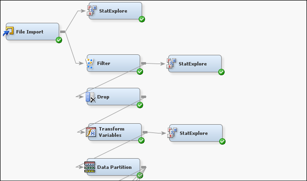
Figure 9: Data preprocessing is done through the filter, drop, transform variables and data partition node.
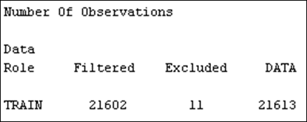
Figure 10: Number of observations excluded from the original dataset.
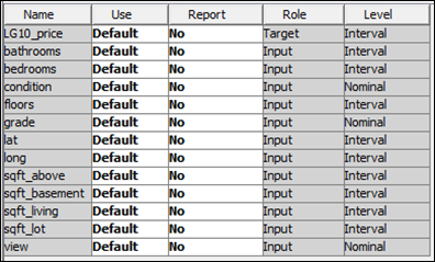
Figure 11: Variables retained for data modelling purposes.
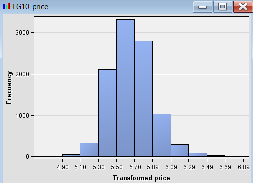
Figure 12: Price data after log transformation.
The identified outliers that contain 0 value for bathrooms and 33
value for bedrooms have been filtered out from the dataset. As shown in Figure 10, this resulted in 11 observations being
excluded, leaving a balance of 21602 observations. One could also perform data
imputation to handle these outliers. However, the remaining sample is large
enough and outlier removal should have minimal impact on the model performance.
In addition, several variables deemed not relevant for this study has been
excluded. This is done to ease the modelling process going forward and avoid having
them mistakenly included in further analysis.
Moreover, the price variable has been transformed using log
transformation because the original distribution is heavily skewed to the
right. Figure 12 shows LG10_price now follows a normal
distribution and will be used as a target variable onwards. It is important to
note when interpreting result from regression modelling that price is
calculated as 10 ^ (predicted value). Lastly, the dataset is partitioned into
training and validation dataset. In this study, 60% of the data is allocated
for training the model, while 40% is used for model validation.
4 Model Construction, Optimization and Validation
For this study, supervise learning and unsupervised learning approach is applied. Some of the supervised learning model used are Regression and Gradient Boosting. Cluster Analysis is used for unsupervised learning.
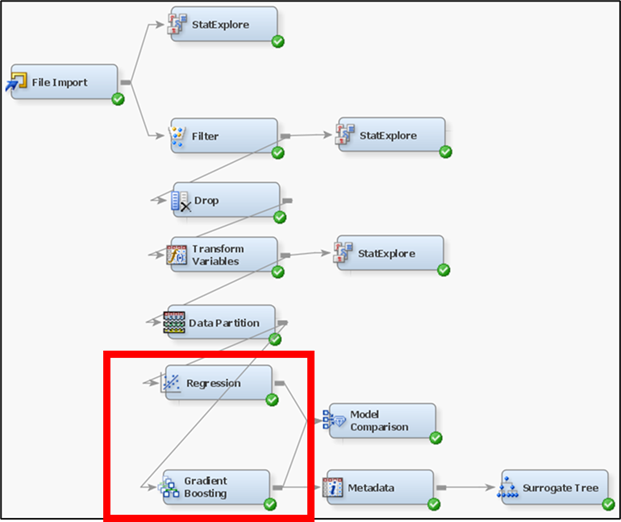
Figure 13: Regression, HP Regression, Gradient Boosting and HP Forest are some of the predictive models employed to estimate house price.
4.1 Regression
This model was built using stepwise selection method. A stepwise method refers to variable selection whereby independent variable is added into the regression equation one step at a time according to its correlation strength against the dependent variable, and its p-value (statistical significance).
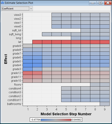
Figure 14: Estimate selection plot showing the sequence of variable addition into model equation.
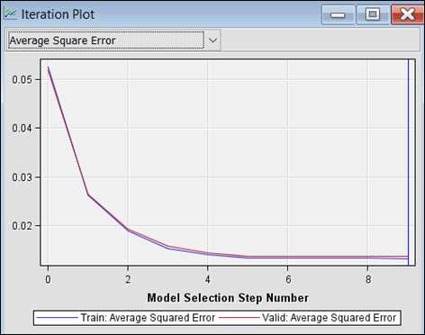
Figure 15: Iteration plot showing Average Square Error against iteration number.
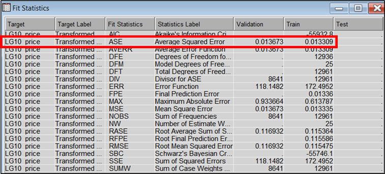
Figure 16:Average Squared Error for the Regression model.
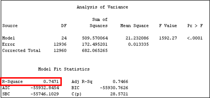
Figure 17: Model summary of the Regression model using Stepwise selection method.
The summary of the Regression model is described as follows:
· The
model iteration plot in Figure
15 shows that the final Regression
model is achieved in step 9. Since variable is added in steps according to the
strength of its influence on the target variable, Figure
14 shows that grade, lat, and sqft_living
are the three variables with the strongest influence on the target variable
– LG10_price.
· From
Figure
17, it is observed the model recorded a
coefficient of determination (R2) value of 0.7471. This means that
74.71% of the variation in LG10_price can be explained by the variables
included in the model. Furthermore, it recorded an Average Squared Error of 0.013673
and 0.013309 for the training and validation dataset, respectively.
4.2 Gradient Boosting
Unlike Regression model, Gradient Boosting (GB) is often considered as a Black Box model due to the complex processes that takes place between the model input and output. It involves an optimization algorithm whereby it is capable of finding the steepest descent in the cost function (error) iteratively when moving from one model to the next. The GB model was tested as an attempt to see if the predicting power of the first Regression model can be approved further.
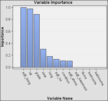
Figure 18: Variable importance determined from Gradient Boosting model.
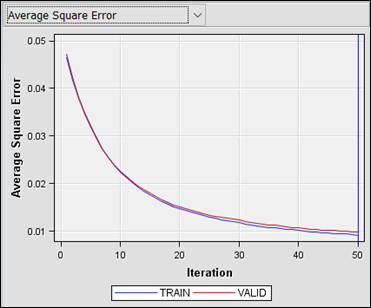
Figure 19: Iteration plot showing Average Square Error against iteration number.
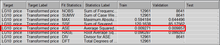
Figure 20: Average Squared Error for the GB model.
The summary of the Regression model is described as follows:
· Figure
18 shows that sqft_living, lat and
grade are three of the most important variables in predicting LG10_price.
Variable importance is exponentially lower for view, long, sqft_lot,
sqft_above and condition. Other remaining variables are considered not
important in predicting the target.
· The
model was run up to 50 iteration using default parameter setting. At iteration
50, the model converges to an Average Square Error of 0.009271 and 0.009857 for
the training and validation dataset, respectively. Note that the R2
value is not computed from SAS Enterprise Miner for GB models, therefore the goodness
of fit is interpreted from the Average Square Error only.
4.3 Model Comparison (Regression and GB model)
The performance for both Supervised Learning models can be compared using the Model Comparison node. The findings are discussed in the following.
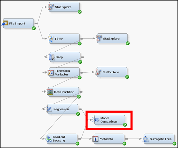
Figure 21: Model comparison node used to evaluate performance between various models.
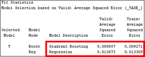
Figure 22: Comparison of Average Squared Error for GB and Regression model.
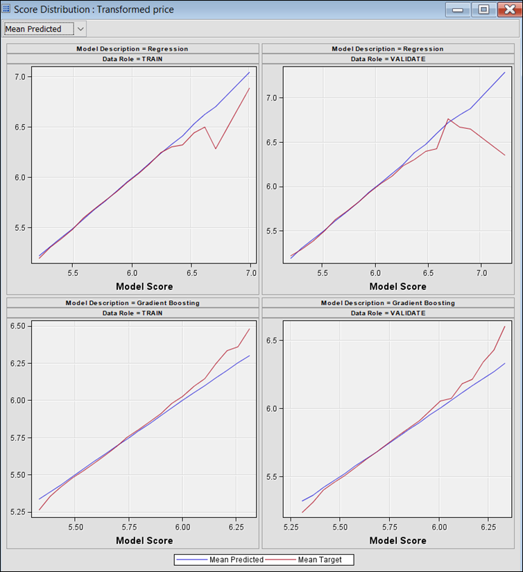
Figure 23: Score distribution plot for Regression and Gb model.
Summary of
model comparison:
· The comparison of Average Squared Error (ASE) for both models is presented in Figure 22. The GB model shows 0.40 % lower ASE for the training dataset, and 0.38 % lower ASE for the validation dataset as compared to the Regression model. Furthermore, there is no overfitting or underfitting issue with both models as ASE is similar for training and validation dataset. GB model is preferred over the Regression model as it yields a lower ASE value overall.
· It can be observed from the score distribution in Figure 23 that GB model slightly overestimate the LG10_price at lower range (5.25 – 5.50) and underestimates it at higher range (6.00 – 6.50). The Regression model on the other hand, shows better model score at lower range, but grossly overestimates at higher range (6.25 – 7.00).
4.4 Cluster Analysis
Cluster analysis is performed to group observations with similar characteristics into various segments or clusters. The observations within a specific cluster should be as homogenous as they can be (minimum dissimilarity) and observations between clusters should be as heterogenous (maximum dissimilarity) as possible. According to a study by Chia et al. (2016), financial factors, distance to amenities, environment, and house features such as size and quality of built is significant in influencing house purchase intention. Therefore, based on our dataset, price_per_sqft_living, sqft_living, bedrooms, lat, long, grade and condition were chosen to reflect the same requirements. Cluster analysis can therefore be used to understand the demand for houses in the county.
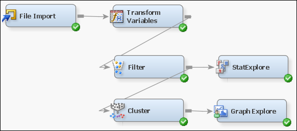
Figure 24 Workflow for Cluster analysis.
Note that a new variable
called price_per_sqft_living is created using the transform variable node. It is useful to segmentize
houses based on this variable as compared to using price because it
shows the price variation in relation to the size aspect of the house which is a
common convention when comparing value of houses with varying sizes.
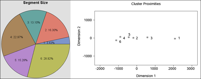
Figure 25:Pie chart showing the segments generated from the cluster analysis with percentage representing number of observations in each segment. Scatter plot showing distances between the segments.
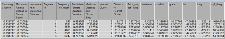
Figure 26:Mean statistics table for the cluster analysis output.
Summary of the Cluster
Analysis:
· There
is no hard and fast rule when it comes to deciding on the number of segments /
clusters. However, the general rule of thumb is maximum dissimilarity between
clusters is preferred and the proportion of the majority of
the clusters should be roughly similar. After trying out with several number of
segments, 6 seem to provide a scenario that in agreement with the general rule
of thumb.
· Segment
1 is the smallest segment holding 3.43% of observations while segment 6 is the
biggest with 28.92% of observations. In terms of distance between the segments (Figure
25), segment 1 is furthest away from
the rest of the segments while segments 2, 4, 5 and 6 are closer to each other.
Segment 3 sits somewhere in between.
· From
the mean statistics table (Figure
26), the houses in each segment can be
profiled using their unique characteristics. For example, houses in segment 1
are the most expensive, having very large sqft_living size, high grade
and the most number of bedrooms. Segment 4 on
the other hand comprise least expensive houses with relatively smaller sqft_living
size and low grade. For segment 6, the houses are expensive but unlike houses
in segment 1, they are much smaller in sqft_living size and have lower number
of bedrooms.
5 Model Interpretation
In this section, model interpretation if performed for Regression model, Gradient Boost model and Cluster Analysis. The purpose and business relevance of each model constructed, as summarized in Table 2, provides the basis for model interpretation.
Table 2: Description and justification of Supervised and Unsupervised learning.
|
Approach |
Models |
Purpose |
Business relevance |
|
Supervised learning |
Regression, Gradient Boosting |
To estimate Price |
Enable developer to set suitable price point according to the market value and avoid overpricing or underpricing |
|
Unsupervised learning |
Cluster analysis |
To group houses that possess similar characteristics into various segments |
Enable developer to identify demand based on different property segments |
5.1 Regression
To interpret the Regression model, one would look at the model coefficients. It provides information on how the target variable – LG10_price changes according to the change in the input variables.
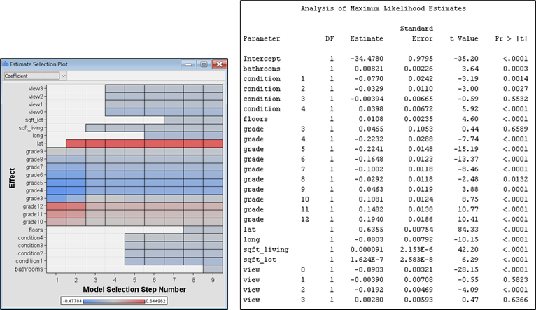
Figure 27: Estimate selection plot and model coefficients for the Regression model.
Interpretation of the
Regression model is described as follows:
· House price in the county varies according to its location. Houses located in the Northern region (high lat), would have a strong positive effect on price. Variation in the East-West direction (lat) have minimal negative impact on price.
· House price increases as view scores increase. View scores of 0, 1, and 2 have a negative effect on price, but view score of 3 will start to affect house price positively. Similar pattern is observed for the condition variable. While condition of 1, 2 and 3 have negative impact, price would start to increase at condition score of 4. Moreover, for the grade variable, scores of 3 – 8 have negative impact on price, but price would start to be positively impacted for grade scores from 9 – 12.
· Number
of floors and bathrooms have a weak positive effect on house
price. The same interpretation can be made for the size of sqft_living
and sqft_lot.
5.2 Gradient Boosting
Since GB is a Black Box model, it is not as straight forward to interpret it as compared to the Regression model. The variable importance plot as shown previously in Figure 18 provides information on which variable affects the model, but it is not exactly understood how these variables affect house price (either positively or negatively, and the magnitude of impact), hence reducing its interpretability. To address this issue, a tree-based model is used as a surrogate to make the output from GB model more interpretable.
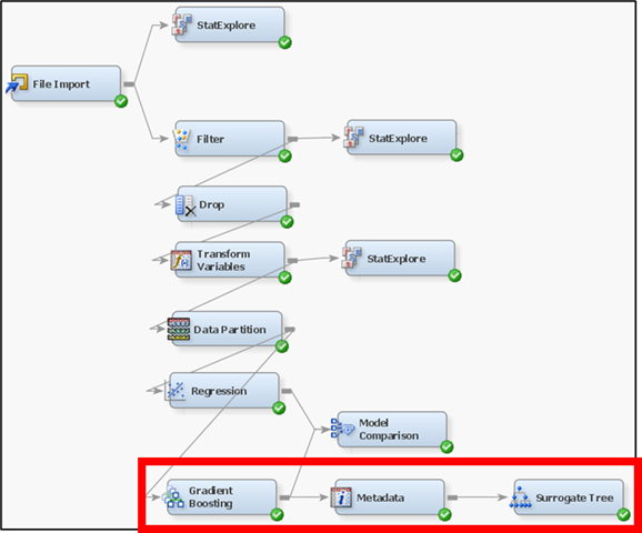
Figure 28: Workflow to improve interpretability of the GB model.
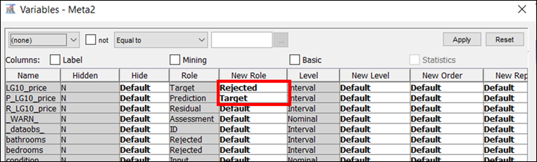
Figure 29: The prediction output from the GB model is set to be the target variable for the surrogate tree.
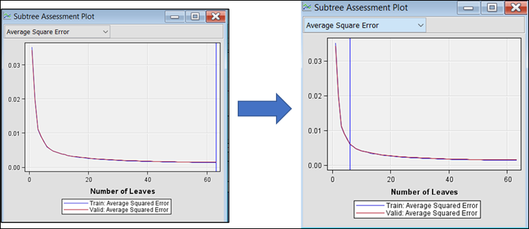
Figure 30: Subtree assessment plot showing the Average Square Error and Number of Leaves.
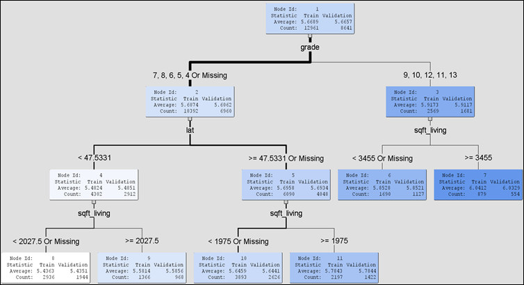
Figure 31: Decision tree based on the output of GB model.
The surrogate model can be created using a Decision Tree node. The target for surrogate model should now be the predicted LG10_Price which is the output of the GB model that is being investigated. This new target can be defined using the Metadata node as shown in Figure 29.
The surrogate model was then run using default parameter setting. It yielded 63 number of leaves with an Average Squared Error of 0.0014 and 0.0015 for the training and validation dataset, respectively. Initial look at the output tree suggest that the tree might be too large which can hinder interpretation. The number of leaves was then pruned / constrained to 6 at 0.006 Average Square Error to come out with a tree that is more interpretable as shown in Figure 31.
|
|
|
|
|
|
|
|
|
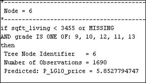
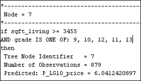
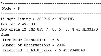
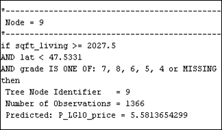
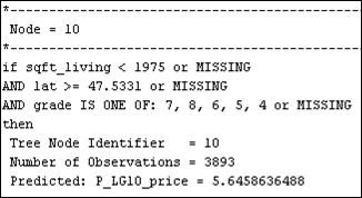
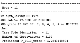
Figure 32: Node rules for the pruned tree at 6 number of leaves.
Interpretation of the Gradient
Boosting model is described as follows:
· Pruning
the surrogate tree to 6 leaf nodes gives an Average Squared Error of 0.006
which is low enough to provide a model with a satisfactory fit. This shows that
with 6 leaf nodes the chosen independent variables (grade, lat, and sqft_living)
fit the predicted LG10_price values with 0.006 Average Squared Error.
· The resulting leave nodes as shown in Figure
32, is quite self-explanatory. Node 6
for example suggests that if a house have a sqft_living of < 3455
with grade scores either 9, 10, 11, 12, or 13 will yield a house price of 10^
(5.852) = $ 712853.03. The lowest predicted house price is recorded under Node
8. Here it is seen that a house with sqft_living < 2027.5, and
latitude position lat < 47.5331 with grade score of less than
4 will sell at a significantly lower price 10^ (5.436) = $ 273073.77. In
general, it can be inferred from the model that an increase in lat, grade
and sqft_living will in increase house price.
· There are quite a number of independent variables that are not included in the pruned surrogate tree. This is because, smaller tree reflects simpler model with a smaller number of variables. Although it enhances interpretability, it could also be viewed as being too generalized. How complex, or simple the model should be would ultimately depend on its ability to meet the business objectives, provided that the misfit or error value is still within a satisfactory level.
5.3 Cluster Analysis
Apart from the mean statistics table (Figure 26), various plots can be generated to help identify each segment with appropriate label. Label should represent the unique characteristics of each segment. For example, a map would help to spatially visualize the location of each segment using its average latitude and longitude position. Scatter plot matrix on the other hand can assist in highlighting unique characteristics of each segment.
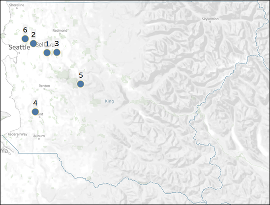
Figure 33: Location of each segment based on its average latitude and longitude position.
|
Segment
1 |
|
|
Segment
2 |
|
|
Segment
3 |
|
|
Segment 4 |
|
|
Segment 5 |
|
|
Segment 6 |
|
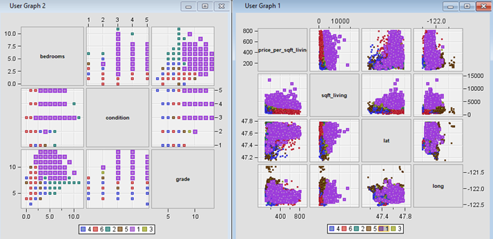
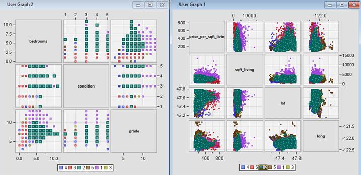
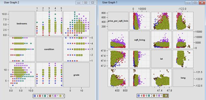
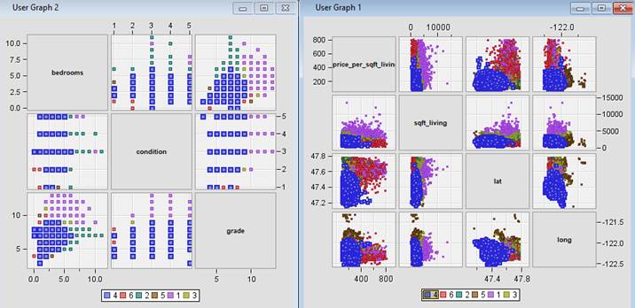
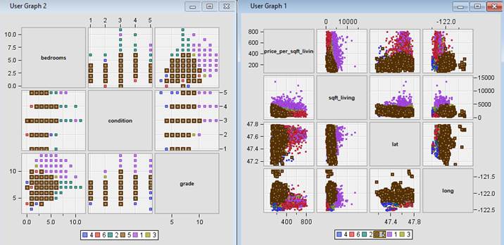
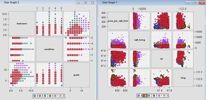
Figure 34: Scatter plot matrix highlighting characteristics of each cluster.
Interpretation of the
Cluster Analysis is described as follows:
· Segment
1 – Suburban Affluent. This segment comprises some of the most
expensive houses in the county. The houses generally have higher grade and condition
score, and they are larger in size averaging around 4636.634 ft2 living.
In terms of location, these are houses that are mostly in the suburban area
(outskirt of Seattle), which is suitable for people who enjoys the convenience
of short commuting distance to the big city, but do not prefer the hustle and
bustle of the city environment. Furthermore, the high price and larger size suggests
that this segment caters to people of the higher income group with larger families.
This segment is the smallest with only 3.43% of the total house sales in the
county and may suggest a low demand.
·
Segment 2 – Urban. This
segment represents houses located in the city. The price and size are
almost half of the houses in Segment 1, but capacity wise, it holds as many
bedrooms on average as the houses in Segment 1. Grade and condition are around
medium to high. Houses in this segment
caters to people of the middle-income group with medium sized families who
enjoys living in the city environment. Segment 2 holds 16.8 % of the houses
sold, and this corresponds to medium demand.
·
Segment
3 – Suburban. The price of houses in this segment are on average
slightly higher than that of Segment 2, but still much lower than Segment 1.
The living size is also between that of Segment 2 and 1. Grade is relatively high,
but the condition of houses is low to medium. The houses in this segment are
suitable for people with larger families who require a bigger living space but
at a more affordable price as compared to Segment 1. However, the commuting
distance to Seattle is slightly increased. 13.10% house sold from this segment
suggest medium demand.
·
Segment 4 – Rural 1. This
segment comprises houses that are located in the rural
area. The average price is 56% and 32% cheaper than houses in Segment 1 and
Segment 2. The living size however is quite small when compared to those two
segments. Grade is generally lower when compared to other segments while
condition is around medium. This segment caters to the lower income group with
smaller family size that do not require regular commute to the city. The demand for houses in this segment is quite
high as 22.97% of house sold in the county is attributed to this segment.
·
Segment 5 – Rural 2. Houses
in this segment are located in another rural area. It
can be distinguished from Segment 4 by its slightly higher price (on average 21%
more) and bigger living size (28% bigger). It is also closer to Seattle as
compared to Segment 4. It is more suitable for buyers with medium sized family.
There is medium demand for houses in this segment (15.25% of house sales).
· Segment
6 – Urban Affluent. Houses in this segment are found in or
near the city centre. Its location is comparable to Segment 2; however, it can
be distinguished by its higher price which is 38% more than that of Segment 2. Despite
the higher price, the living size is almost halved of those houses in Segment 2.
Number of bedrooms is also lower with average of 2 bedrooms. Houses in this
segment are suitable for high-income professionals working in the city centre
with small sized family. There is very high demand for houses in this segment
as it recorded 28.92% of the total house sales in the county.
6 Discussion and Conclusion
Predictive model for implementation. The choice of the model should be based on its performance (measure of fit) and interpretability. Therefore, the Gradient Boosting model is recommended because it yielded a 0.4 % lower Average Squared Error compared to the Regression model. In addition to that, despite being a black box model, it has been demonstrated that output from GB model can still be interpreted using a tree based surrogate model. The level of model complexity can be controlled by pruning the tree. The lower the number of leaves, the simpler the model is and the easier it is to interpret. However, the model risk to be too generalized if it is too simple with very few numbers of input variables. Therefore, there is a need to find the right balance between interpretability without compromising the model fit which can satisfy the business objective.
Housing market segmentation. Using cluster analysis, 6 segments in the housing market has been identified. The segments are Urban, Urban Affluent, Suburban, Suburban Affluent, Rural 1, and Rural 2. Each segment carries a unique characteristic based on its average price per ft2, living size, location, condition, and grade. Demand for houses with certain attributes can be estimated from the number of houses sold in each segment. In general, there to be high demand for houses in the Rural 1 and Urban Affluent segment. The Urban, Suburban and Rural 2 segment sees a medium demand while the Suburban Affluent segment suggests the lowest demand.
Business application. Seattle houses the headquarter of one of the biggest technology company in the world – Amazon. According to the Seattle Office of Planning and Community, Development (2017) due to the booming tech industry, the city is expected to add 120,000 people and 115,000 jobs Between 2015 and 2035. Furthermore, 73.5% of its population is in the labor force which is 13% higher than the country’s average. The median income of $92,263 is also 46% higher than the country’s average (United States Census Bureau, 2019). It is therefore not surprising that the Urban Affluent segment recorded the highest house sales transaction – 28.92% of the total house sales in the whole county.
The developer is then recommended to target the Urban Affluent segment as the data strongly suggests that there is high demand for it. The developer should build houses with attributes that is in line with the segment profile. For example, there should be 2-3 bedrooms, with around 1433 ft2 of living space, built in the city center for fast commute between home and the city center, and built with medium condition and medium quality in mind. The predictive model can then be used to make data-driven decision in setting the house price and reduce the risk of overpricing or underpricing.
To increase the profit margin, the developer may choose to expand the size indicator (living space) as the predictive model shows that square foot living affect house price positively. However, undeveloped land in the city center is quite scarce and this option may not be as viable. The developer can instead opt to increase the grade and condition score of the house by sourcing quality materials and workmanship and ensure that condition of the house is well maintained post-construction.
Furthermore, incorporating smart-home system to enhance security, enable home management insights for energy efficiency and overall improvement on convenience is also recommended. By doing so the developer can offer a unique value proposition to the market and the houses can be offered at a higher price compared to the segment average.
In conclusion, a combination of supervised
and unsupervised learning approach has been applied in this study. The Gradient
Boosting model was chosen over Regression model for house price prediction as
it recorded lower Average Squared Error and provide solution that is
interpretable for the business. Moreover, cluster analysis was performed to analyze
demand based on the different house characteristics. The predictive model and
output from cluster analysis were used in combination to better meet the
business objectives.
7
References
San Ong, T. (2013). Factors Affecting the
Price of Housing in Malaysia, Finance and Banking (JEIEFB) An Online
International Monthly Journal.
Taltavull
Paz, P. (2003). Determinants of housing prices in Spanish cities, Journal of
Property Investment & Finance. doi: 10.1108/14635780310469102.
University of Regina. Overview
of the KDD Process. Available at http://www2.cs.uregina.ca/~dbd/cs831/notes/kdd/1_kdd.html [Accessed 23 March 2021].
Chia, J., Harun, A.,
Kassim, A. W. M., Martin, D., & Kepal, N. (2016). Understanding factors
that influence house purchase intention among consumers in Kota Kinabalu: an
application of buyer behavior model theory. Journal of Technology Management
and Business, 3(2).
Seattle Office of Planning and
Community, Development (2017). City of
Seattle Growth and Livability Report. Available at https://www.seattle.gov/Documents/Departments/OPCD/Livability/Growth%20and%20Livability%20Report.pdf [Accessed 6 May 2021].
United States Census Bureau (2019). QuickFacts Seattle city, Washington; United States. Available at https://www.census.gov/quickfacts/fact/table/seattlecitywashington,US/PST045219. [Accessed 6 May 2021].